Space Sextics from Blowing up 8 Points in the Plane
Let \(\mathcal{P}:=\{P_1,P_2, ... ,P_8\}\) be a configuration of eight \(k\)-rational points in \(\mathbb{P}^2_k\) that are in general position (i.e. no three points on a line, no six points lie on a conic, … ). A space sextic can be costructed by blowing up \(\mathbb{P}^2_k\) at \(\mathcal{P}\) as follows: The space of plane cubics through all eight points has a basis \(\{u,v\}\). The space of ternary sextics vanishing doubly on \(\mathcal{P}\) is spanned by \(\{u^2,uv,v^2,w\}\) for some ternary sextic \(w\). Finally, the \(7\) dimensional space of plane nonics vanishing triply on \(\mathcal{P}\) has a basis of the form \(\{u^3,u^2v,uv^2,v^3,uw,vw,r\}\). Now consider the folowing two commutative diagrams:
where
and \(\pi\) is the projection to the first three coordinates. The image of \(\psi\) is a del Pezzo surface \(X\) of degree one and \(\pi(X)\) is branched along a curve \(C\) of weighted degree \(6\). \(\phi(C)\) gives the space sextic curve we are looking for.
This magma script has functions for
constructing the equations of the space sextic \(C\) on the singular quadric \(V(x_0x_2-x_1^2)\) in \(\mathbb{P}^3\) with coordinates \((x_0:x_1:x_2:x_3)\),
computing the equations of the 120 tritangents corresponding to the odd theta characteristics of \(C\),
counting the number of totally real tritangents among the aforementioned 120 tritangents.
Constructing the curve from 8 points in the plane
Here is an example of constructing the equations of the space sextic using the script:
> load "tritangentsDelPezzo.m";
Loading "tritangentsDelPezzo.m"
> C, Q, Qcone, u,v,w := ConstructBranchCurve(P2,Lpts);
> GetCanonicalModelFromCone(P3,Qcone);
Curve over Rational Field defined by
x0^3 - 3760834826206762527557287188288729260167/1119922155716145169377094085056\
 7691600*x0^2*x1 + 141552652437042555549114924032152995336827074471919477190\
 78196300963041615838399/501690253945559083310453733748482882278176079339671\
 173558423975010842240000*x0^2*x2 - 9927931984893787389599334476275489640543\
 19386581587319008484582193868490014035035697/260560080023627545770709742065\
 095396330581431570648685904518890879297740620800000*x0*x1*x2 +
 295949760423754696798756117011126749568134984082889603931751950793947951229\
 7258129462493263/1753820310028092141088962911721649117190558650505354504951\
 67536821336873396174995456000000*x0*x2^2 +
 413369171703172931882637477234342870018652351690788491752745182350837722883\
 0074463689488355533579/5465231465838740355499545039334846690334322992589445\
 63693701142675492347052181905173381120000000*x1*x2^2 +
 680883293904434043957012256183833646454794322485630775105526394049788345220\
 5754341851228732212123560321/6131045312673769744537059212750900925047020626\
 6722385484372641052444808831497748057131965638246400000000*x2^3 +
 6176718872646818036383544135023027682567/1119922155716145169377094085056769\
 1600*x0^2*x3 - 731033044183230897033991487541342280622665013530199/40046447\
 465259602273717119550228535361416720000*x0*x1*x3 +
 147439016554244537129198416558311743153598375950755408073219/44925194029899\
 27689183770981709813718459910703078400000*x0*x2*x3 -
 90919826913401332085920779572288913971921546284102996559598288581/419985871\
 90015518397995834048773096135845582802370607104000000*x1*x2*x3 -
 188482995353418836738361225127256942858006901842133304310106207869441519/31\
 41010498088731797398143474839985724893764652503438101985361920000000*x2^2*x\
 3 + 32531379537612802839217/17048691612407520000*x0*x3^2 -
 5430766485552823657815928122383/478142149380265335513600000*x1*x3^2 +
 145189769998906312971295258607755364083/17879762288041493219876081664000000\
 *x2*x3^2 - 361737607193370320227304146619/478142149380265335513600000*x3^3,
x1^2 - x0*x2
We will now explain the general procedure and all functions involved.
First, we need to check that the given set of eight points in the plane are in general position. The input of the following function is a list L of eight points and it returns true, if they are in general position:
function CheckGeneralPosition(L)

        // We assume that L is a non-empty list of points in the projective plane.
        assert #L ne 0;
        assert Type(L[1]) eq Pt;
        P2 := Scheme(L[1]);
        assert IsProjective(P2) and IsAmbient(P2) and Dimension(P2) eq 2;

        // Check that the points are in general position
        k := BaseRing(P2);
        _<x,y,z> := PolynomialRing(k,3);
        pts := {ChangeUniverse(Eltseq(pt), k) : pt in L};

        // No coincident points
        if #L ne #pts then return false; end if;

        // No three lie on a line
        for S in Subsets(pts,3) do
                mons := Monomials((x+y+z));
                M := Matrix(k,3,3,[[Evaluate(m,pt) : pt in S] : m in mons]);
                if Determinant(M) eq 0 then return false; end if;
        end for;

        // No six lie on a conic
        for S in Subsets(pts,6) do
                mons := Monomials((x+y+z)^2);
                M := Matrix(k,6,6,[[Evaluate(m,pt) : pt in S] : m in mons]);
                if Determinant(M) eq 0 then return false; end if;
        end for;

        // Any cubic through all 8 is non-singular at each point
        for s in pts do
                mons := Monomials((x+y+z)^3);
                M := Matrix(k,10,8,[[Evaluate(m,pt) : pt in pts] : m in mons]);
                N := Matrix(k,10,3,[[Evaluate(Derivative(mon,1),s),
                                        Evaluate(Derivative(mon,2),s),
                                        Evaluate(Derivative(mon,3),s)] : mon in mons]);

                MN := HorizontalJoin(M,N);
                if Rank(MN) ne 10 then return false; end if;
        end for;

        return true;
end function;
Next, we require a function that computes the cubics vanishing singly and sextics vanishing doubly at eight points. The following function is more general. Given the ambient space X, a positive integer n, and a list [<Pi, mi>] of points with multiplicities, it returns the linear system of degree n homogenous polynomials vanishing at each Pi with multiplicity mi. Later, this function will also be used to compute the tritangent planes.
function LinearSystemFromPoints(X,n,Lpts)
        L := LinearSystem(X,n);
        for elt in Lpts do
               L := LinearSystem(L,elt[1],elt[2]);
        end for;

        return L;
end function;
The space sextic curve that we would like to compute can be also viewd as the image of the plane nonic vanishing triply at \(\mathcal{P}\), under the map \(\eta = \phi \circ \varphi\). After computing the plane nonic \(C\), as done in the function “ConstructBranchCurve”, one could diretly use the map \(\eta\) to get the canonical model of the curve in \(\mathbb{P}^3\). However, for the sake of performance, we break it into multiple steps.
First, we embed the plane curve into \(\mathbb{P}(1:1:2)\) using the function “GetConeModel”. Then we compute the plane model and the cone model of the curve using the function “ConstructBranchCurve”. Finally, from the cone model we determine the equations of the curve in \(\mathbb{P}^3\) using the function “GetCanonicalModelFromCone”.
function GetConeModel(Q,u,v,w)

        R<x,y,z> := Parent(u);
        k := BaseRing(Parent(u));
        A<T> := PolynomialRing(k);
        _<W> := PolynomialRing(A);

        L6Sections := [ u^i*v^(6-i) : i in [0 .. 6]] cat [ w*u^i*v^(4-i) : i in [0 .. 4]] cat [w^2*u^i*v^(2-i) : i in [0 .. 2]] cat [w^3];
        image_basis:= [ T^i : i in [0 .. 6]] cat [ W*T^i : i in [0 .. 4]] cat [W^2*T^i : i in [0 .. 2]] cat [W^3];

        mons := Monomials((x+y+z)^18);
        coeff_matrix := Matrix(k, [[MonomialCoefficient( s, mon) : mon in mons] : s in L6Sections]);

        Qsq := Q^2;
        vecQsq := Vector(k, [MonomialCoefficient( Qsq, mon) : mon in mons]);

        img_coeffs, N := Solution(coeff_matrix, vecQsq);
        assert Dimension(N) eq 0;

        return &+[ img_coeffs[i] * image_basis[i] : i in [1 .. #image_basis]];
end function;
INPUTS:
Q – defining polynomial of the singular nonic \(C\) on the projective plane
u,v – The cubics generating the linear system of cubics through the eight points
w – A sextic such that <u^2, uv, v^2, w> generates the sextics vanishing doubly at each point
OUTPUT:
The cone model of the space sextic which is a curve of weighted degree 6 in \(\mathbb{P}(1:1:2)\) with coordinates (S:T:W) Where S is set to be 1.
function ConstructBranchCurve(P2, Lpts);

        assert IsProjective(P2) and IsAmbient(P2) and Dimension(P2) eq 2 and IsField(BaseRing(P2));
        R := CoordinateRing(P2);

        if Type(Lpts) eq SeqEnum then

                assert #Lpts eq 8 and &and[Type(pt) eq Pt : pt in Lpts];
                if not CheckGeneralPosition(Lpts) then error "Points not in general position."; end if;

                if &and[Scheme(pt) eq P2 : pt in Lpts] then
                         L3 := LinearSystemFromPoints(P2, 3, [< pt, 1> : pt in Lpts]);
                         L6 := LinearSystemFromPoints(P2, 6, [< pt, 2> : pt in Lpts]);
                else
                         // This is the case our points define a cluster over K.
                         calP := &join [Cluster(pt) : pt in Lpts];
                         calP := Scheme(P2, [R ! f : f in DefiningEquations(calP)]);
                         calPtimes2 := Scheme(P2, DefiningIdeal(calP)^2);

                         L3 := LinearSystem(P2, 3);
                         L3 := LinearSystem(L3, calP);
                         L6 := LinearSystem(P2, 6);
                         L6 := LinearSystem(L6, calPtimes2);
                end if;
        else
                error "ConstructBranchCurve requires a list of points as input.";
        end if;

        u := Sections(L3)[1];
        v := Sections(L3)[2];

        L3Squared := LinearSystem(P2, [u^2,u*v,v^2]);
        w := Sections(Complement(L6,L3Squared))[1];

        J := JacobianMatrix([u,v,w]);
        Q := Determinant(J);
        C := Curve(P2,Q);

        Qcone := GetConeModel(Q,u,v,w);

        return C, Q, Qcone, u,v,w;
end function;
INPUTS:
P2 – ambient projective space. Must be \(\mathbb{P}^2\) over a field K.
Lpts – either
a list of eight points in P2(K).
a list of eight points in P2(K^sep). The set of eight points should define a cluster defined over K.
OUTPUTS:
C – a singular model of the branch curve in P2
Q – the defining equation of C
Qcone – the defining equation of the space sextic curve in a cone P(1:1:2)
u,v – the cubics generating the linear system of cubics through the eight points
w – a sextic such that <u^2, uv, v^2, w> generates the sextics vanishing doubly at each point
function GetCanonicalModelFromCone(P3, Qcone)
        k := BaseRing(P3);
        _<x0,x1,x2,x3> := CoordinateRing(P3);
        R<t> := PolynomialRing(k);
        coeffs := Coefficients(Qcone);
        mons := [R ! m : m in Monomials(Qcone)];
        q := x0*x2-x1^2;

        F := CoordinateRing(P3) ! (x1^6*(&+[Evaluate(coeffs[i], x0/x1)
                                * Evaluate(mons[i], x0*x3/x1^2)
                                : i in [1 .. #coeffs]]));
        X := Curve(Scheme(P3, [q, F]));

        // X is not defined properly since the "inverse" of P112 --> P3 is a bit delicate.

        comps := IrreducibleComponents(X);
        C := [co : co in comps | IsReduced(co)][1];
        return Curve(C);
end function;
INPUTS:
P3 – ambient projective space. Must be \(\mathbb{P}^3\) over a field K
Qcone – The defining equation of the branch curve in a cone \(\mathbb{P}(1:1:2)\)
OUTPUT:
The defining equations of the space sextic curve in \(\mathbb{P}^3\) with coordinates \((x_0:x_1:x_2:x_3)\): A quadric \(x_1^2-x_0x_2\) and a cubic form.
Computing the tritangents to space sextic constructed by 8 points
There are two approaches to compute the tritangent planes to the space sextic curve that comes from blowing up the plane in 8 points. One option, knowing the defining equations of the curve, would be a similar approach as in the generic case. Since our quadric is fixed, we can use a particular parametrization of the curve on \(\mathbb{P}(1:1:2)\) to simplify the process.
Here is an examplary function for computing 120 tritangent planes to \(C\). However, based on our experiments, it is much slower compared to the next approach. Hence it merely serves as a proof of concept and is thus omitted in our uploaded script.
function CComputeTritangents(C)

        k := BaseField(C);
        P3<x0,x1,x2,x3> := AmbientSpace(C);
        de := DefiningEquations(C);
        q := [e : e in de | Degree(e) eq 2][1];
        f := [e : e in de | Degree(e) eq 3][1];

        // Equations to detect when a univariate polynomial of degree 6 is a square
        P6 := AffineSpace(k,7);
        c := AffineSpace(k,4);
        _<t> := PolynomialRing(CoordinateRing(c));
        g := &+[c.i*t^(i-1) : i in [1 .. 4]];
        square_map := map< c->P6 | Coefficients(g^2)>;
        VarSqrs := Image(square_map);
        P6k := ChangeRing(P6,k);

        // Assert the quadric is normalized
        assert q eq x1^2-x0*x2;

        // Solve for the tritangents
        R1<s,t,u> := PolynomialRing(k,3);
        phi1 := hom< CoordinateRing(P3) ->  R1 | [s^2, s*t, t^2, u]>;

        P3dual<a,b,c>:= AffineSpace(k,3);
        R2 := CoordinateRing(P3dual);
        R3<S,U> := PolynomialRing(R2,2);
        phi2 := hom<R1 -> R3 | [S,1,U]>;

        F := phi2(phi1(f));
        h := a*S^2 + b*S + c + U;

        Fs := Resultant(F,h,U);
        maptoS := map<P3dual -> P6k | [Coefficient(Fs, S, i) : i in [0 .. 6]]>;

        Fu := Resultant(F,h,S);
        maptoU := map<P3dual -> P6k | [Coefficient(Fu, U, i) : i in [0 .. 6]]>;

        Tgt_scheme := (VarSqrs @@ maptoS) meet (VarSqrs @@ maptoU);
        assert IsCluster(Tgt_scheme);

        assert Degree(Tgt_scheme) eq 120;
        Tgt_pts := PointsOverSplittingField(Tgt_scheme);

        // **********************************************************************
        // Base field, curve, and ambient projective space redefined.

        // Modify the base field of objects.
        k := Parent(Random(Tgt_pts)[1]);
        P3<x0,x1,x2,x3> := ChangeRing(P3, k);
        C := Curve(Scheme(P3, [f,q]));
        Tgt_list := [ p[1]*x0 + p[2]*x1 + p[3]*x2 + x3 : p in Tgt_pts];

        return k, P3, C, Tgt_list;
end function;
INPUT:
a space sextic curve C
OUTPUTS:
k – field of definition
P3 – ambient projective space, which must be \(\mathbb{P}^3_k\)
C – the curve
Tgt_list – a list of 120 tritangent planes in \(\mathbb{P}^3\) with coordinates \((x_0,x_1,x_2,x_3)\).
The second approach is to find the plane curves that are corresponding to the tritangent planes. It also has the added benefit that it makes computing the contact points, and thus determining the total realness of the tritangents, much easier.
To be more precise, there are 120 pairs of curves in \(\mathbb{P}^2\) that map to \(240\) exceptional curves on \(X\). Each pair of exceptional curves project to one of the 120 curves of weighted degree 2 in \(\mathbb{P}(1:1:2)\). The 120 tritangent planes to the space sextic are the images of these 120 curves under the map \(\phi\). As before, instead of directly using the map \(\eta\) and computing the images of the pairs under it, we pass through \(\mathbb{P}(1:1:2)\) for better performance.
> load "tritangentsDelPezzo.m";
Loading "tritangentsDelPezzo.m"
> Tgt_list := AllTritangentsInP3();
> #Tgt_list;
120
> Random(Tgt_list);
x0 - 2804950608070416595115857729/148876661112727945085430190800*x1 -
  4178871991462012777298163250319251/5567129596048015833231397058020992000*x2
  + 32885237017579120020664013329/148876661112727945085430190800*x3
As before, we will explain the general procedure and all functions involved.
The following piece of code is used to create lists with elements of the form [<Pi, mi>] where Pi is a point and mi is its multiplicity. The input for “MakeMultiplicityMap” is a list of size 8 with integer elements. For example, given a list Lpts of 8 points, multmap1(Lpts) is a list of 28 elements. Each element is again a list consisting of two points with multiplicity 1 and the remaining six points with multiplicity 0. It corresponds to a line through a pair of points.
function MakeMultiplicityMap(mults)
        multperms := { [mults[f[i]] : i in [1 .. #mults]] : f in Permutations({1 .. #mults}) };

        // Remove the multiplicites corresponding to the image under Bertini.
        for x in multperms do
              minusX := [2-y : y in x];
              // Note that destructive operations do not apply to the for loop condition, but they
              // do apply to the variable `multperms`. This is why we need the if statement.
              if x in multperms then Exclude(~multperms, minusX); end if;
        end for;

        function MultMap(Lpts)
              assert #Lpts eq #mults;
              return { [<Lpts[i], mp[i]> : i in [1 .. #Lpts]] : mp in multperms};
        end function;
        return MultMap;
end function;

multmap0 := MakeMultiplicityMap([1,0,0,0,0,0,0,0]);
multmap1 := MakeMultiplicityMap([1,1,0,0,0,0,0,0]);
multmap2 := MakeMultiplicityMap([1,1,1,1,1,0,0,0]);
multmap3 := MakeMultiplicityMap([2,1,1,1,1,1,1,0]);
The following two functions are used to make a cone model of each tritangent plane from one of its corresponding plane curves.
The first function is just used in second function, so here you see the input and output for the main function “GetConeCurve”:
function GetConeTritangent(F, u,v,w, A)
        R<x,y,z> := Parent(u);
        k := BaseRing(Parent(u));
        _<W> := PolynomialRing(A);
        T := A.1;

        L2Sections := [ u^i*v^(2-i) : i in [0 .. 2]] cat [w];
        image_basis:= [ T^i : i in [0 .. 2]] cat [ W ] ;

        mons := Monomials((x+y+z)^6);
        coeff_matrix := Matrix(k, [[MonomialCoefficient( s, mon) : mon in mons] : s in L2Sections]);

        vecf := Vector(k, [MonomialCoefficient( F, mon) : mon in mons]);

        img_coeffs, N := Solution(coeff_matrix, vecf);
        assert Dimension(N) eq 0;

        return &+[ img_coeffs[i] * image_basis[i] : i in [1 .. #image_basis]];
end function;


function GetConeCurve(P2, n, Qcone, S, u, v, w : descendToRationals:=false)
        if n ne 0 then
           L := LinearSystemFromPoints(P2,n,S);
           assert #Sections(L) eq 1;
           f := Sections(L)[1];
           minusS := [ <a[1], 2-a[2]> : a in S];
        else
           f := 1;
           minusS := [ <a[1], 2+a[2]> : a in S];
        end if;

        L := LinearSystemFromPoints(P2, 6-n,minusS);
        assert #Sections(L) eq 1;
        g := Sections(L)[1];

        // The polynomial defining the exceptional curve times its Bertini conjugate.
        // We normalize to ensure that at least one coefficient of F is rational.
        F := f*g; F := F/LeadingCoefficient(F);

        if descendToRationals then
           k  := Rationals();
           P2 := ChangeRing(P2, k);
           try
                F  := Parent(u) ! ChangeRing(F, k);
           catch e
                // In the case that F is not defined over Q, we know that the tritangent is not
                // defined over R. In this case, we return "false" along with a dummy
                // discriminant value.
                return false, TRITGT_NOT_RAT;
           end try;
        end if;

        return GetConeTritangent(F, u, v, w, BaseRing(Parent(Qcone)));
end function;
INPUTS:
P2 – ambient projective space. Must be \(\mathbb{P}^2\) over a field K.
n – degree of the plane curve corresponding to the tritangent plane
Qcone – the defining equation of the space sextic curve on the cone P(1:1:2)
S – a list [<Pi, mi>] of points with multiplicites to creat the plane curve
u,v – the cubics generating the linear system of cubics through the eight points
w – a sextic such that <u^2, uv, v^2, w> generates the sextics vanishing doubly at each point
OUTPUT:
a cone model of the tritangent plane which is a polynomial of weighted degree 2 in \(\mathbb{P}(1:1:2)\) with coordinates \((S:T:W)\) where \(S\) is set to be 1.
Finally, the following function returns a list of 120 tritangent planes to the space sextic curve in \(\mathbb{P}^3\) with homogeneous coordinates \((x_0,x_1,x_2,x_3)\). It does not have a direct input and uses the functions that are defined before to first construct the cone model of 120 tritangent planes and then transfer them to \(\mathbb{P}^3\)
function AllTritangentsInP3()

        C, Q, Qcone, u,v,w := ConstructBranchCurve(P2,Lpts);

        Tritangents8 :=    [ GetConeCurve(P2, 0, Qcone, S, u, v, w) : S in multmap0(Lpts)];
        Tritangents28 :=   [ GetConeCurve(P2, 1, Qcone, S, u, v, w) : S in multmap1(Lpts)];
        Tritangents56 :=   [ GetConeCurve(P2, 2, Qcone, S, u, v, w) : S in multmap2(Lpts)];
        Tritangents56_2 := [ GetConeCurve(P2, 3, Qcone, S, u, v, w) : S in multmap3(Lpts)];
        Tgt_list := Tritangents8 cat Tritangents28 cat Tritangents56 cat Tritangents56_2;


        // Put tritangent equations and the curve in P3
        P3<x0,x1,x2,x3> := ProjectiveSpace(k,3);
        Tritangents := [];
        for tt in Tgt_list do
             cox3 := Coefficient(Coefficient(tt,1),0);
             cox2 := Coefficient(Coefficient(tt,0),0);
             cox1 := Coefficient(Coefficient(tt,0),1);
             cox0 := Coefficient(Coefficient(tt,0),2);
             ttcoeffs := [cox0,cox1,cox2,cox3];
             tgteq := &+[P3.i*ttcoeffs[i] : i in [1 .. 4]];
             Include(~Tritangents, tgteq);
        end for;
        return Tritangents;
end function;
The number of totally real tritangent planes:
There are 120 pairs of curves in the plane map to the 240 exceptional curves on \(X\) under the map \(\psi\). Each pair corresponds to a tritangent plane to the space sextic \(C\), i.e. two exceptional curves that are images of one pair under \(\psi\) map to a tritangent plane via \(\phi \circ \pi\).
A tritangent plane is called totally real if it is cut out by a real form and has all the three contact points real. For a tritangent plane to be totally real, all of the intersection points of the two plane curves in the corresponding pair has to be real. To be more precise, each pair intersect in exactly three points, out of \(\mathcal{P}\). The corresponding tritangent plane is totally real if the three points are real.
In the following figure, the conic through \(P_{i_1}, \ldots, P_{i_5}\) matches the quartic vanishing at \(\mathcal{P}\) and doubly at the three other points. Their intersection in \(\mathbb{P}^2 \setminus \mathcal{P}\) consists of three points.
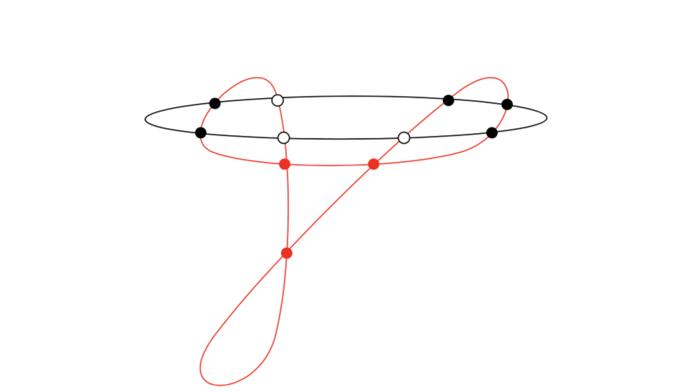
Here \(\mathcal{P}\) is the set of all of the filled points.
The uploaded magma script can check how many of the 120 exceptional pairs yield totally real tritangents (for more examples, see the next section on experimental results):
> load "tritangentsDelPezzo.m";
Loading "tritangentsDelPezzo.m"
> TotRealTritCount(P2,P2,Lpts,Lpts);
120
We will now explain the general procedure and all functions involved.
The following function checks whether the 8 tritangents corresponding to the blow-ups at eight points are totally real or not.
function IsTotallyRealTangentCone(C,P : assertReal:=true)
        // We assume that P does not lie on the hyperplane at infinity.
        assert Scheme(P) eq C;

        P2<x,y,z> := AmbientSpace(C);
        k := BaseRing(P2);
        tc := TangentCone(C,P);

        assert Degree(tc) eq 3;

        if assertReal then
              assert (k eq Rationals() or IsNumberField(k));
        end if;

        if not IsOrdinarySingularity(P) then
              // The only way this happens is if some of the contact points with C coincide.
              // In particular, they must all be real
           return true, 0;
        end if;

        F := Evaluate(DefiningEquation(tc), [x,y,0]);

        // Define the number field over which the tangent directions split.
        R<t> := PolynomialRing(BaseRing(P2));

        if Coefficient(F, x , 3) ne 0 then
                f := Evaluate(F, [t,1,0]);
        else
                f := Evaluate(F, [1,t,0]);
        end if;

        return (Discriminant(f) ge 0), Discriminant(f);
end function;
INPUTS:
C – the model of the space sextic curve on the projective plane
P – a point on the plane model. One of the eight original points chosen in the construction
OUTPUT:
True or False that determines whether the corresponding tritangent is totally real or not.
For the remaining 112 of the 120 tritangent planes we use the following functions. The first function is used in the second one, which is why we will only list the input and output of the second function.
function OptimizedCheckCone(P2, Qcone, F , u, v, w )

        ell := GetConeTritangent(F, u, v, w, BaseRing(Parent(Qcone)));
        assert Degree(ell) eq 1;

        g := BaseRing(Parent(Qcone)) ! Evaluate(Qcone, -Coefficient(ell,0)/Coefficient(ell,1));

        // g should be a square up to leading coefficient, so we want to take the square root.
        h := GCD(g, Derivative(g));
        assert Degree(ExactQuotient(g, h^2)) eq 0;
        assert LeadingCoefficient(h) eq 1;

        if Degree(h) lt 1 then return true; end if;
            assert Degree(h) lt 4;
        return Discriminant(h) ge 0, Discriminant(h), ell;
end function;

function CheckConeCurve(P2, n, Qcone, S, u, v, w : descendToRationals:=false)
        L := LinearSystemFromPoints(P2,n,S);
        assert #Sections(L) eq 1;
        f := Sections(L)[1];

        minusS := [ <a[1], 2-a[2]> : a in S];
        L := LinearSystemFromPoints(P2, 6-n,minusS);
        assert #Sections(L) eq 1;
        g := Sections(L)[1];

        // The polynomial defining the exceptional curve times its Bertini conjugate.
        // We normalize to ensure that at least one coefficient of F is rational.
        F := f*g; F := F/LeadingCoefficient(F);

        if descendToRationals then
              k  := Rationals();
              P2 := ChangeRing(P2, k);

              try
                    F  := Parent(u) ! ChangeRing(F, k);
              catch e
                    // In the case that F is not defined over Q, we know that the tritangent is not
                    // defined over R. In this case, we return "false" along with a dummy
                    // discriminant value.
                    return false, TRITGT_NOT_RAT;
              end try;
        end if;

        return OptimizedCheckCone(P2, Qcone, F, u, v, w );
end function;
INPUTS:
P2 – ambient projective space. Must be \(\mathbb{P}^2\) over a field K.
n – degree of the plane curve corresponding to the tritangent plane
Qcone – the defining equation of the space sextic curve on the cone P(1:1:2)
S – a list [<Pi, mi>] of points with multiplicites to creat the plane curve
u,v – the cubics generating the linear system of cubics through the eight points
w – a sextic such that <u^2, uv, v^2, w> generates the sextics vanishing doubly at each point
OUTPUT:
True or False that determines whether the corresponding tritangent is totally real or not
Finally, the function for counting the number of totally real tritangents:
function TotRealTritCount(P2,P2K,Lpts,Lrealpts)

       C, Q, Qcone, u,v,w := ConstructBranchCurve(P2,Lpts);

       //check if each tritangent corresponding to blow ups at points is real
       if Lrealpts ne [] then
           Lrealpts := [P2 ! pt : pt in Lrealpts];
           pointconds:= [IsTotallyRealTangentCone(C, C ! pt) : pt in Lrealpts];
       else
           pointconds := [];
       end if;


       // Check if each of the lines gives rise to totally real tritangent
       lineconds := [CheckConeCurve(P2K, 1, Qcone, S, u, v, w :  descendToRationals:=true) : S in multmap1(Lpts)];

       //    --    each of the conics gives rise to totally real tritangent
       conicconds:= [CheckConeCurve(P2K, 2, Qcone, S, u, v, w :  descendToRationals:=true) : S in multmap2(Lpts)];

       //    --    each of the cubics gives rise to totally real tritangent
       cubicconds:= [CheckConeCurve(P2K, 3, Qcone, S, u, v, w :  descendToRationals:=true) : S in multmap3(Lpts)];

       // Count the number of totally real tritangents

       numtotsreal :=   #[l : l in pointconds | l eq true]
                      + #[l : l in lineconds | l eq true]
                      + #[l : l in conicconds | l eq true]
                      + #[l : l in cubicconds | l eq true];

       return numtotsreal;

end function;
INPUTS:
P2 – ambient projective space. Must be \(\mathbb{P}^2\) over a field K
Lpts – a list of eight points in P2(K)
Lrealpts – a list containing the real points of Lpts
P2K – projective space of dimension 2 over Cyclotomic Field of order 4 and degree 2
OUTPUT:
the number of totally real tritangent planes to the space sextic cunstructed by blowing up P2 at Lpts
Experimental results
A space sextic with 120 totally real tritangents
Here is a configuration of points in \(\mathbb{P}^2_\mathbb{Q}\) for which the blow up of the plane gives rise to a space sextic with all 120 tritangent planes being totally real. This is the default example that is included in the uploaded script.
k := Rationals();
P2 := ProjectiveSpace(k,2);
P3<x0,x1,x2,x3> := ProjectiveSpace(k,3);

Lpts := [ [1, 0 , 0], [0 , 1 , 0], [0 , 0 , 1], [1 , 1 , 1],
          [10 , 11 , 1], [27 , 2 , 17], [-19 , 11 , -12], [-15 , -19 , 20] ];
Lpts := [P2 ! pt : pt in Lpts];

TotRealTritCount(P2,P2,Lpts,Lpts);

> 120
Special point configurations
The previous example was eight real points in the plane, which yields a space sextic with five connected components and 120 real tritangents. More generally, a configuration of eight points with \(5-s\) complex conjugated pairs, \(s\in\{0,1,2,3,4\}\), gives rise to a space sextic with \(s\) ovals and \(2^{s+2}\) real tritangents. However, the number of totally real tritangents might vary broadly.
The following files comprise of various point configurations, yielding different numbers of totally real tritangents. They represent the information that Table 1 in arXiv:1712.06274 was generated from:
point configurations yielding space sextics with a single ovalpoint configurations yielding space sextics with three ovals
Their numbers of totally real tritangents can be verified with our uploaded script as follows:
> Lpts :=  [ Eltseq(Vector(K, [1*I, 1-1*I, 0])),
  Eltseq(Vector(K,  [-1*I, 1+1*I, 0])),
              Eltseq(Vector(K,[2-1*I , -3-1*I , 3+1*I])),
              Eltseq(Vector(K,[2+1*I , -3+1*I , 3-1*I])),
              Eltseq(Vector(K, [2-1*I , 1-1*I , -2-1*I])),
  Eltseq(Vector(K, [2+1*I , 1+1*I , -2+1*I])),
  Eltseq(Vector(K,[4*I , -1*I , 4])),
        Eltseq(Vector(K,[-4*I , 1*I , 4]))];
> Lpts := [P2K ! pt : pt in Lpts];
> Lrealpts := [];
> TotRealTritCount(P2,P2K,Lpts,Lrealpts);
0