Space Sextics from Intersections of Quadrics and Cubics
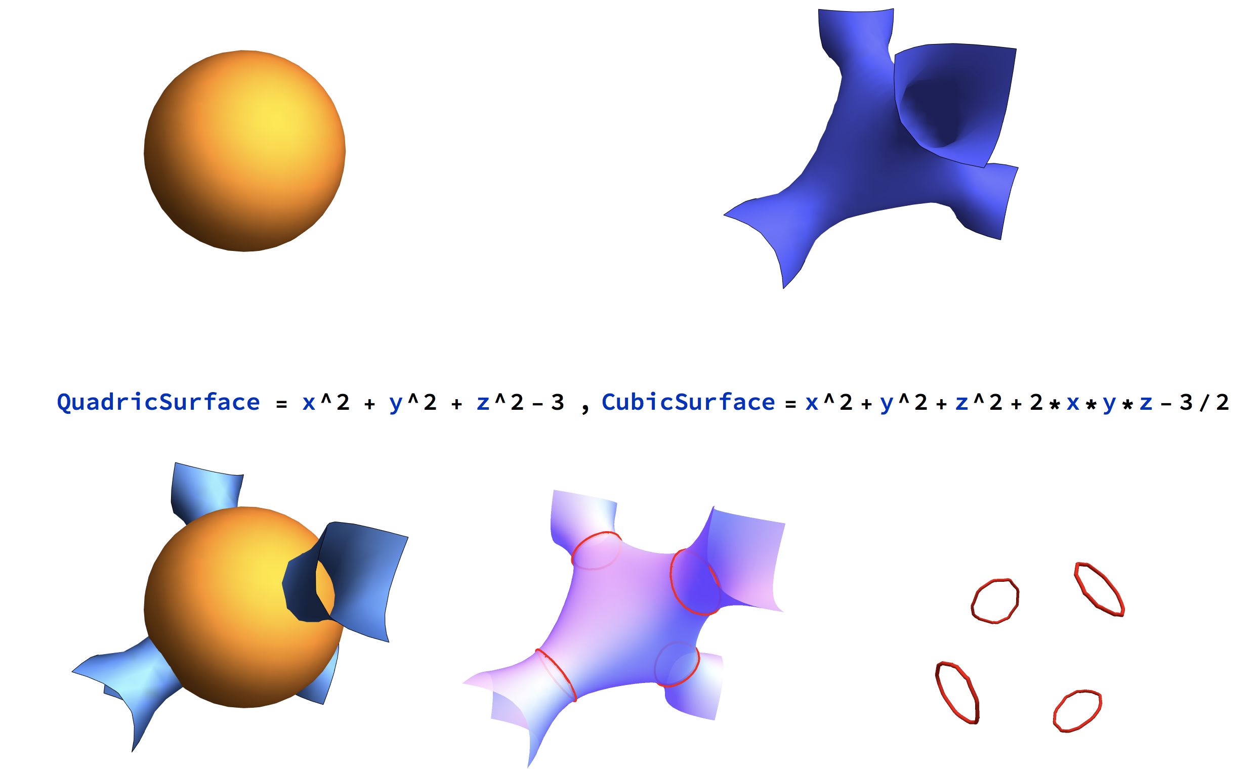
A generic sextic is the intersection of a quadric and a cubic surface. Given a quadric \(Q=V(f)\) and a cubic \(K=V(g)\), \(f,g\in\mathbb C[x_0,\ldots,x_3]\), we will now construct and solve the tritangent ideal, an ideal in \(\mathbb C[u_0,\ldots,u_3]\) whose solutions are all planes \(H=V(u_0x_0+\ldots+u_3x_3)\) that are tritangent to the space sextic \(C=Q\cap K\).
The magma script can be downloaded here. It begins with defining:
the base field K, which has to be either the rational numbers of an algebraic extension thereof, over which \(f\) and \(g\) are defined,
a field CC of complex numbers with fixed high precision over which the tritangents are computed numerically,
a field CCout of complex numbers with fixed low precision over which the solutions are returned.
_<l> := PolynomialRing(Rationals());
K<l> := NumberField(l^2-3);
P<x0,x1,x2,x3> := PolynomialRing(K,4);
f := x0^2+x1^2+x2^2-25*x3^2;
g := (x0+l*x3)*(x0-l*x1-3*x3)*(x0+l*x1-3*x3)-2*x3^3;

CC := ComplexField(250);
_<l> := PolynomialRing(CC);
ll := Roots(l^2-3)[2][1];
roundingMap1 := hom<K->CC|Evaluate(l,ll)>;

CCout:= ComplexField(10);
roundingMap2 := hom<CC->CCout|>;
What follows is split up in three parts
Multiple root loci of multiplicity \((2,2,2)\)
As precomputation, consider the projective space \(\mathbb P^6\) whose points \((a_0,\ldots,a_6)\in\mathbb P^6\) are the binary sextics
Inside \(\mathbb P^6\), construct the threefold of squares of binary cubics:
whose defining prime ideal is minimally generated by 45 quartics in \(a_0,a_1,a_2,a_3,a_4,a_5,a_6\):
S<a0,a1,a2,a3,a4,a5,a6> := PolynomialRing(Rationals(),7);
R<b0,b1,b2,b3,t> := PolynomialRing(Rationals(),5);
phi := hom<S->R|Coefficients((b0+b1*t+b2*t^2+b3*t^3)^2,t)>;
ker := MinimalBasis(PolyMapKernel(phi));
Constructing the tritangent ideal
Now we shift our attention to our prescribed quadric \(f\) and cubic \(g\) in \(K[x_0,\ldots,x_3]\) over \(K\) which cut out our space sextic \(C\).
Consider the parametrized plane \(h:=u_0 x_0+\ldots+u_3 x_3\) over the transcendental field \(K(u_0,\ldots,u_3)\). The aim is find generators of the tritangent ideal, equations in \(u_0,\ldots,u_3\) which guarantee that \(h\) is tritangent to \(C\).
Ru<u0,u1,u2,u3> := PolynomialRing(K,4);
Ku<u0,u1,u2,u3> := FieldOfFractions(Rabcd);
Pu<x0,x1,x2,x3> := PolynomialRing(Kabcd,4);
h := u0*x0+u1*x1+u2*x2+u3*x3;
iota := hom<P->Pu|[x0,x1,x2,x3]>;
f := iota(f);
g := iota(g);
This is done by projecting the intersection of the sextic and the plane onto the coordinate axes and forcing the projections to be three double points. For sake of performance, we rely on resultants rather on eliminations.
The projection onto the \(x_0,x_1\) axis, or rather the coefficients of the univariate degree 6 polynomial which cut the 6 points in the projection, can be obtained two ways:
f3 := Evaluate(f,[x0,x1,x2,(-u0*x0-u1*x1-u2*x2)/u3]);
g3 := Evaluate(g,[x0,x1,x2,(-u0*x0-u1*x1-u2*x2)/u3]);
r32,den := ClearDenominators(Resultant(f3,g3,x2));
r32 := r32*den;
C32 := Coefficients(Evaluate(r32,[x0,1,0,0]));
or
f2 := Evaluate(f,[x0,x1,(-u0*x0-u1*x1-u3*x3)/u2,x3]);
g2 := Evaluate(g,[x0,x1,(-u0*x0-u1*x1-u3*x3)/u2,x3]);
r23,den := ClearDenominators(Resultant(f2,g2,x3));
r23 := r23*den;
C23 := Coefficients(Evaluate(r23,[x0,1,0,0]));
We do both in order to gain additional elements in our tritangent ideal, and repeat the process with all other axes:
f3 := Evaluate(f,[x0,x1,x2,(-u0*x0-u1*x1-u2*x2)/u3]);
g3 := Evaluate(g,[x0,x1,x2,(-u0*x0-u1*x1-u2*x2)/u3]);
r32,den := ClearDenominators(Resultant(f3,g3,x2));
r32 := r32*den;
C32 := Coefficients(Evaluate(r32,[x0,1,0,0]));
r31,den := ClearDenominators(Resultant(f3,g3,x1));
r31 := r31*den;
C31 := Coefficients(Evaluate(r31,[x0,0,1,0]));
r30,den := ClearDenominators(Resultant(f3,g3,x0));
r30 := r30*den;
C30 := Coefficients(Evaluate(r30,[0,x1,1,0]));

f2 := Evaluate(f,[x0,x1,(-u0*x0-u1*x1-u3*x3)/u2,x3]);
g2 := Evaluate(g,[x0,x1,(-u0*x0-u1*x1-u3*x3)/u2,x3]);
r23,den := ClearDenominators(Resultant(f2,g2,x3));
r23 := r23*den;
C23 := Coefficients(Evaluate(r23,[x0,1,0,0]));
r21,den := ClearDenominators(Resultant(f2,g2,x1));
r21 := r21*den;
C21 := Coefficients(Evaluate(r21,[x0,0,0,1]));
r20,den := ClearDenominators(Resultant(f2,g2,x0));
r20 := r20*den;
C20 := Coefficients(Evaluate(r20,[0,x1,0,1]));

f1 := Evaluate(f,[x0,(-u0*x0-u2*x2-u3*x3)/u1,x2,x3]);
g1 := Evaluate(g,[x0,(-u0*x0-u2*x2-u3*x3)/u1,x2,x3]);
r13,den := ClearDenominators(Resultant(f1,g1,x3));
r13 := r13*den;
C13 := Coefficients(Evaluate(r13,[x0,0,1,0]));
r12,den := ClearDenominators(Resultant(f1,g1,x2));
r12 := r12*den;
C12 := Coefficients(Evaluate(r12,[x0,0,0,1]));
r10,den := ClearDenominators(Resultant(f1,g1,x0));
r10 := r10*den;
C10 := Coefficients(Evaluate(r10,[0,0,x2,1]));

f0 := Evaluate(f,[(-u1*x1-u2*x2-u3*x3)/u0,x1,x2,x3]);
g0 := Evaluate(g,[(-u1*x1-u2*x2-u3*x3)/u0,x1,x2,x3]);
r03,den := ClearDenominators(Resultant(f0,g0,x3));
r03 := r03*den;
C03 := Coefficients(Evaluate(r03,[0,x1,1,0]));
r02,den := ClearDenominators(Resultant(f0,g0,x2));
r02 := r02*den;
C02 := Coefficients(Evaluate(r02,[0,x1,0,1]));
r01,den := ClearDenominators(Resultant(f0,g0,x1));
r01 := r01*den;
C01 := Coefficients(Evaluate(r01,[0,0,x2,1]));
To force that all projections are three double points, we substitute our coefficients into the previously generated multiple root loci:
iota := hom<Pu->Ru|[0,0,0,0]>;
C32 := iota(C32);
C31 := iota(C31);
C30 := iota(C30);
psi32 := hom<S->Ru|C32>;
C32 := psi32(ker);
psi31 := hom<S->Ru|C31>;
C31 := psi31(ker);
psi30 := hom<S->Ru|C30>;
C30 := psi30(ker);

C23 := iota(C23);
C21 := iota(C21);
C20 := iota(C20);
psi23 := hom<S->Ru|C23>;
C23 := psi23(ker);
psi21 := hom<S->Ru|C21>;
C21 := psi21(ker);
psi20 := hom<S->Ru|C20>;
C20 := psi20(ker);

C13 := iota(C13);
C12 := iota(C12);
C10 := iota(C10);
psi13 := hom<S->Ru|C13>;
C13 := psi13(ker);
psi12 := hom<S->Ru|C12>;
C12 := psi12(ker);
psi10 := hom<S->Ru|C10>;
C10 := psi10(ker);

C03 := iota(C03);
C02 := iota(C02);
C01 := iota(C01);
psi03 := hom<S->Ru|C03>;
C03 := psi03(ker);
psi02 := hom<S->Ru|C02>;
C02 := psi02(ker);
psi01 := hom<S->Ru|C01>;
C01 := psi01(ker);
Finally, we gather all equations in \(u_0,\ldots,u_3\) and restrict ourselves onto an affine chart, say \(u3\neq 0\). This gives us a zero-dimensional ideal with exactly 120 solutions over the algebraic closure of \(K\).
C := C32 cat C31 cat C30 cat C23 cat C21 cat C20 cat C13 cat C12 cat C10 cat C03 cat C02 cat C01;
Su<u0,u1,u2> := PolynomialRing(K,3);
pi := hom<Ru->Su|[u0,u1,u2,1]>;
I := ideal<Su|pi(C)>;
SetVerbose("Groebner",1);
// VarietySizeOverAlgebraicClosure(I); // omit this step if too costly
Solving the tritangent ideal
The final part of the script revolves around computing the solutions of the previously computed tritangent ideal. We start by computing a radical decomposition, which gives us a decomposition into triangular sets whose univariate element is irreducible (warning: in many example this is the most costly step):
RD := RadicalDecomposition(I);
Having this, we compute the solutions of each factor numerically through simple back-substitution:
CCu<u0,u1,u2> := PolynomialRing(CC,3);
phi := hom<Su->CCu|roundingMap1,u0,u1,u2>;
RRD := [phi(Generators(rd)) : rd in RD];

realRoots := [];
complexRoots := [];
for H in RRD do
  _,h := IsUnivariate(H[3]);
  R2 := Roots(h);
  for rr2 in R2 do
    r2 := rr2[1];
    _, h := IsUnivariate(Evaluate(H[2],[u0,u1,r2]));
    R1 := Roots(h);
    for rr1 in R1 do
      r1 := rr1[1];
      _, h := IsUnivariate(Evaluate(H[1],[u0,r1,r2]));
      R0 := Roots(h);
      for rr0 in R0 do
        r0 := rr0[1];
        if (Im(r0) eq 0 and Im(r1) eq 0 and Im(r2) eq 0) then
          realRoots := Append(realRoots,[r0,r1,r2,1]);
        else
          complexRoot := Append(complexRoots,[r0,r1,r2,1]);
        end if;
      end for;
    end for;
  end for;
end for;
Finally, we trim our results to the desired precision for the output:
realRoots_out := [[roundingMap2(r[1]),roundingMap2(r[2]),roundingMap2(r[3])]: r in realRoots];
complexRoots_out := [[roundingMap2(r[1]),roundingMap2(r[2]),roundingMap2(r[3])]: r in complexRoots];
Visualizing space sextics and their tritangents
This mathematica notebook takes
a space sextic, in form of a quadric and a cubic,
its real tritangents \((u_0,u_1,u_2,u_3)\) as previously computed,
and
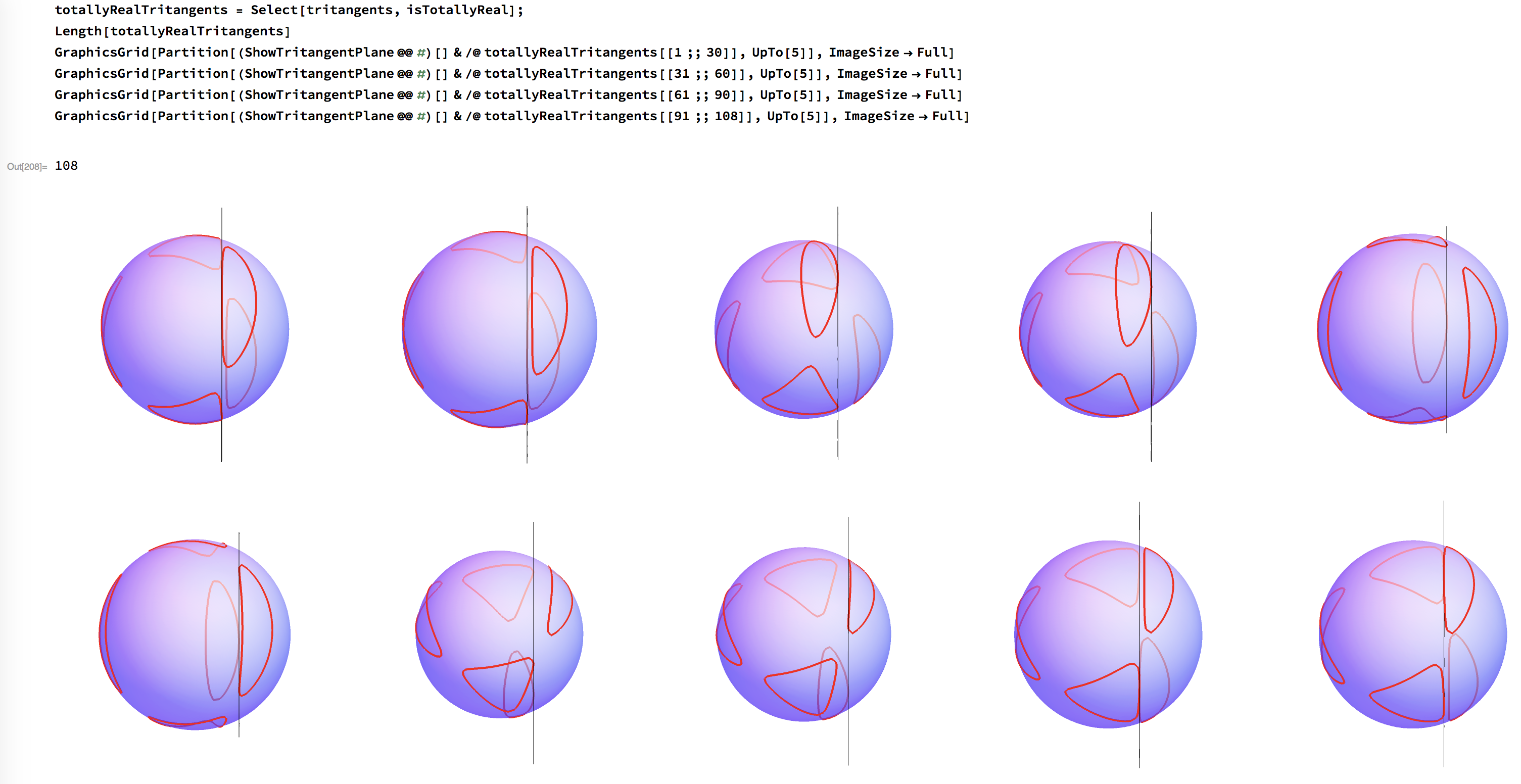
distinguishes between totally real tritangents and tritangents with non real intersection points,
visualizes both types of tritangents seperately.
By default, it contains Emch’s curve and its 120 real tritangents computed through the previous magma script. (Note that the number of tritangents per visualization grid should not exceed 50 for sake of stability.)